Inflow performance

5.1.4 Inflow#

The section provides information about the well inflow parameters that are used for building the IPR (Inflow Performance Relationship) curve.

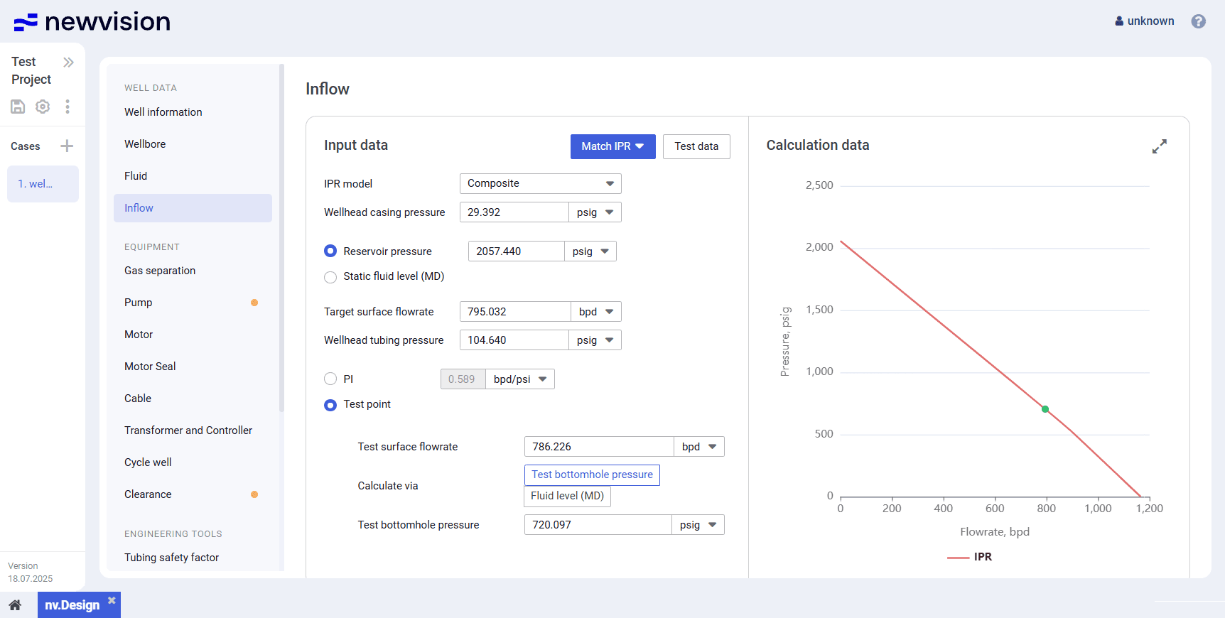
The section consists of two panes:

• Input data
• Calculation data

Select image to enlarge

5.1.4.1 Input Data#

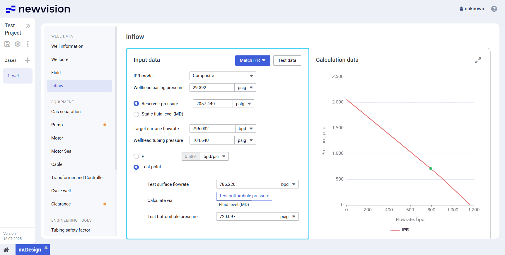
The pane contains the well parameters used for the IPR construction.

Select image to enlarge

The IPR configuration depends on the model that is used for calculation. The choice of the model should be determined by the reservoir type, well operating conditions, analysis goals, and available data.

For details on the IPR configuration, see Calculating IPR.

You can select one of the following models from the IPR model list:

Composite

This model combines several inflow models and is applied under complex operating conditions: high water cut (above 40–50%), multiphase flow (oil, water, gas), varying inflow regimes, and reservoir heterogeneity. 
This approach requires a more comprehensive dataset but provides a more realistic estimate of well performance, especially when bottomhole pressure significantly deviates from bubble point pressure and phase transitions or inflows from different reservoir zones occur.

Vogel Model

This model assumes homogeneous flow (typically oil) and is most effective when bottomhole pressure is below bubble point pressure with minimal water production. It accounts for gas liberation due to pressure drop and provides reliable inflow prediction for undersaturated reservoirs. 
However, the model’s accuracy decreases with high water cut. In this case, the composite model is preferred. The PI model is not suitable under these conditions, as it fails to account for multiphase effects.

PI (Productivity Index)

This model is based on a linear relationship between flow rate and pressure drawdown and is applicable only when bottomhole pressure is above bubble point pressure and water cut is low. 
In the presence of gas release or increasing water production, the model becomes unreliable because it does not reflect phase changes or increased flow resistance under multiphase flow conditions.

The calculation can be based either on the reservoir pressure value or, if it is unavailable, on the static fluid level. You can also select between calculation based on the productivity index ( PI ) and a set of custom parameters ( Test point ). For details, see Calculating IPR.

5.1.4.2 Calculation Data#

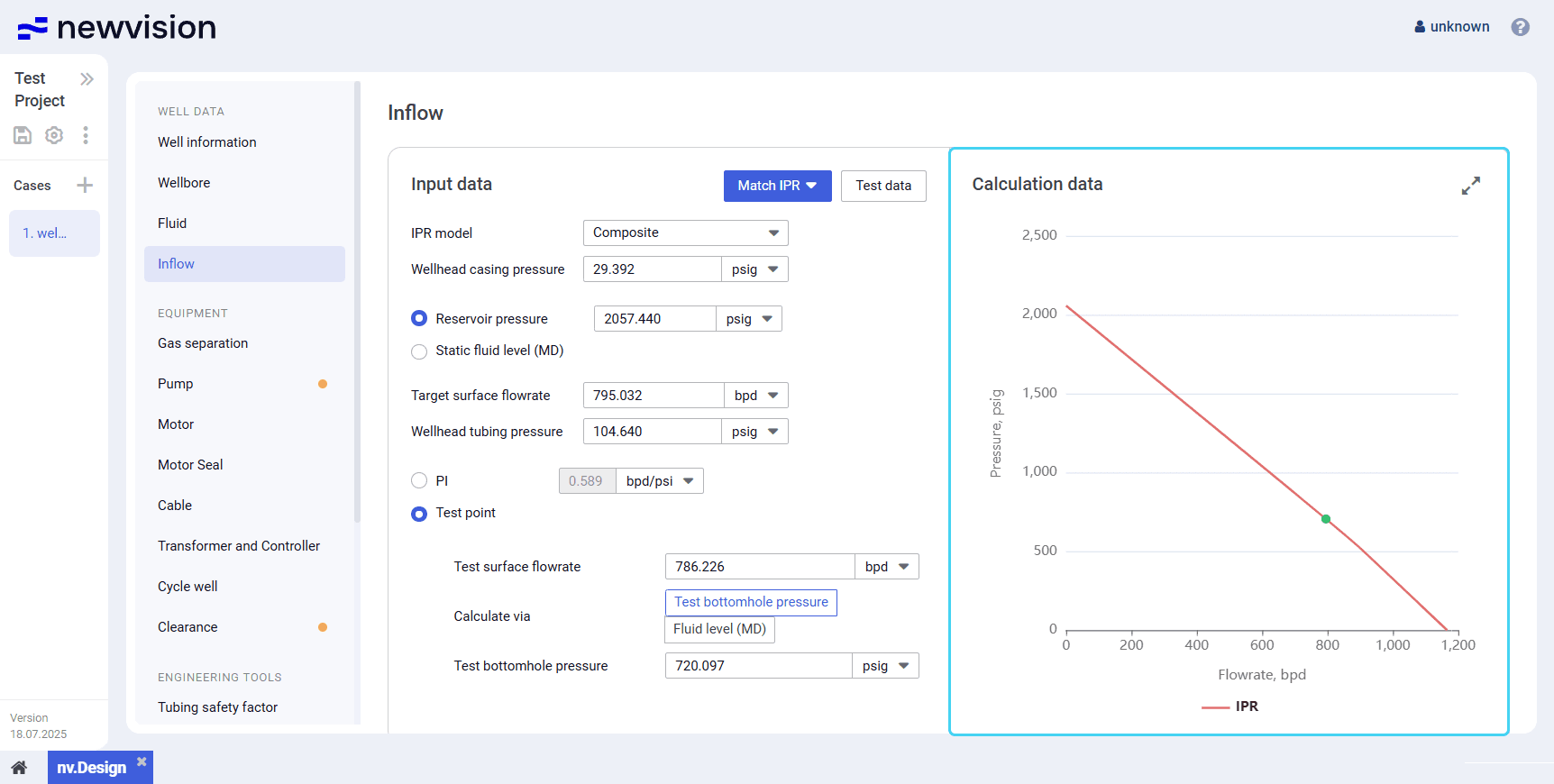
The pane contains the IPR curve constructed based on the parameter values entered in the Input data pane.

Select image to enlarge

You can expand the pane to full screen or collapse it back to the original size using the Expand ( ) / Collapse ( ) buttons located in the upper-right corner of the pane.

Calculating IPR

To configure deviation survey parameters and run a calculation, perform the following actions:

1. Open the nv.design module. 
   For details on navigation in the system, see System Interface.

2. In the left part of the working area, in the list of the module sections, click Inflow . 
   To the right of the list, the Inflow section opens. 
    

   Select image to enlarge

3. In the upper-right corner of the Input data pane, click Test data . 
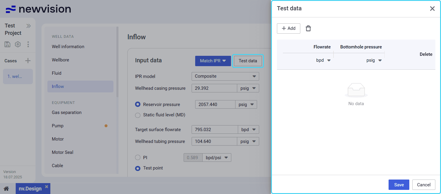
   The Test data window opens. 
    

   Select image to enlarge

4. In the window, enter actual values of the flow rate and corresponding bottom hole pressures obtained during well tests:

   a. Above the table, click Add ( ) . 
   A new row appears in the table.

   In the new row, double-click values in the Flowrate and Bottomhole pressure columns and enter the desired values.

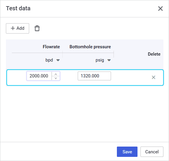   Select image to enlarge

   c. Repeat Steps 1–2 for all available measurements.

   Note  The more measurements you add, the more accurate results the calculation provides.

   Scroll horizontally to view a wide table.

   d. (Optional)

   To edit an entry, double-click the desired value and make necessary changes.

   To delete an entry, select it in the table, and then, above the table, click Delete ( ) , or click the cross icon ( ) in the Delete column.

   e. At the bottom of the window, click Save .

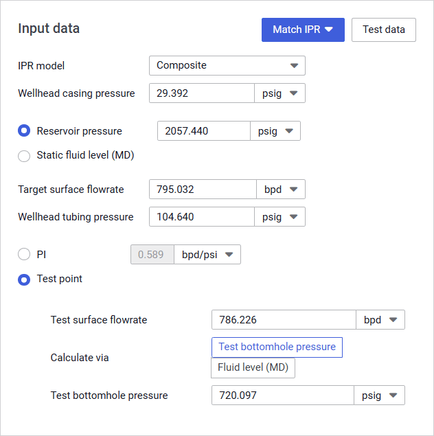
5. At the top of the Input data pane, from the IPR model list, select the appropriate model: Composite , Vogel , or PI . For description of these models, see Inflow. 
    

   Select image to enlarge

6. In the Wellhead casing pressure field, enter the desired value.
7. Select the parameter that will be used for the calculation: Reservoir pressure or, if it is unavailable, Static fluid level (MD) .
8. (Optional) If the Static fluid level (MD) option is selected, fill in the Wellhead casing pressure and Static fluid level (MD) fields.
9. In the Target surface flowrate and Wellhead tubing pressure fields, enter the desired target values.
10. Select one more parameter based on which the calculation will be performed: productivity index ( PI ) or a set of custom parameters ( Test point ).

11. Depending on the option selected at the previous step, perform one of the following actions:

    (For PI ) In the PI field, enter the productivity index value.

    (For Test point ) Fill in the Test surface flowrate field, select the desired Calculate via option, and fill in the rest of the fields.

12. In the upper-right corner of the Input data pane, click Match IPR and select PI from the drop-down menu. 
    In the Calculation data pane, the IPR curve is matched to the actual data and configured calculation parameters.
13. To save changes, in the left part of the module, click Save ( ) under the name of the current project.