Wellbore configuration, deviation survey and heat transfer
Wellbore configuration, deviation survey and heat transfer: 5.1.2 Wellbore The Wellbore section provides information about the downhole equipment, well profile, and heat…
On this page
5.1.2 Wellbore#
The Wellbore section provides information about the downhole equipment, well profile, and heat transfer. It consists of three tabs:
5.1.2.1 Wellbore configuration#
On the Wellbore Configuration tab, you can configure tubing and casing parameters, such as their top and bottom depths (MD), number of stages, and diameters.
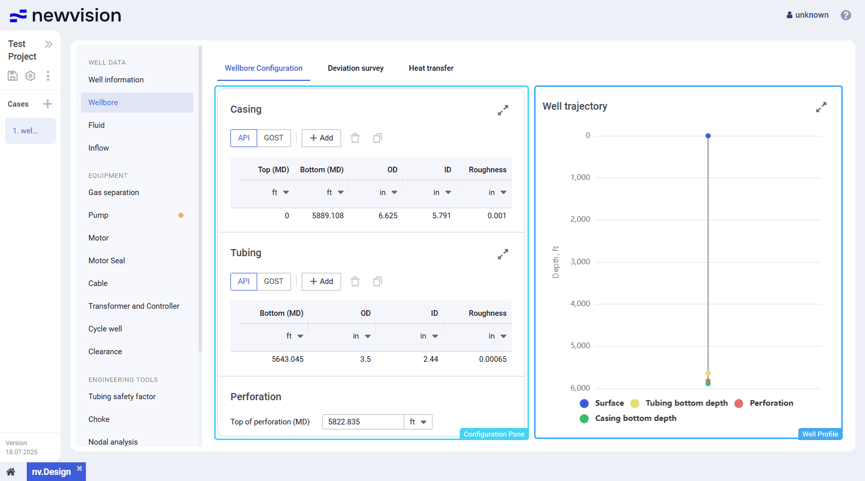
The tab consists of two panes:
- Configuration pane in the left part of the tab.
- Well profile in the right part of the tab.
 Select image to enlarge
Configuration Pane
The pane contains three groups of parameters: Casing , Tubing , and Perforation .
The Casing and Tubing groups contain tables with corresponding parameters. Each row in the table corresponds to one casing or tubing stage.
Both tables provide the following controls:
API/GOST
Provides the ability to select the set of standard pipe sizes, API (American Petroleum Institute standard) or GOST (Russian national standard), that prescribes the tubing and casing outer and inner diameters.
Add (  )
)
Adds a new row to the table for entering the casing or tubing stage parameters at the specified depth. For details, see Configuring Casing and Tubing Data.
You can enter data to the tables manually or paste it to a new row from another source using the Ctrl+V shortcut. The source table must have the same column configuration as the target one. The pasted entries are automatically sorted by depth.
For example, you can try copying the data from the following table:
| Top (MD) | Bottom (MD) | OD | ID |
| 0 | 8690 | 7 | 6.276 |
| 8400 | 11320 | 4.5 | 3.92 |
| 0 | 7150 | 2.875 | 2.441 |
 | Note The header row must not be copied from the source table. |
Delete (  )
)
Deletes the selected row from the table.
Clone (  )
)
Creates a copy of the selected row.
Expand (  ) / Collapse (
  )
)
Expands the parameter group to full screen or collapses it back to the original size.
The Perforation group contains only one parameter, Top of perforation (MD) .
Well Profile
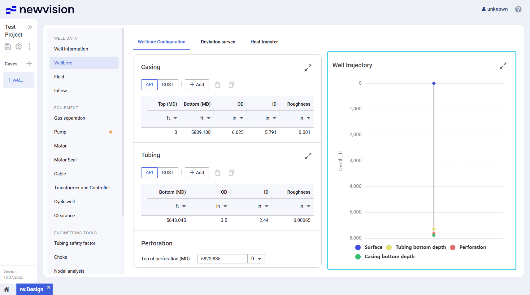
The pane contains the well profile that is built based on the data entered in the left part of the section (see description above).
 Select image to enlarge
On the profile, depths are displayed as markers of different color.
To show or hide a marker, click its name under the profile.
You can also expand the pane to full screen or collapse it back to the original size using the Expand ( ) / Collapse ( ) buttons located in the upper-right corner of the pane.
5.1.2.1.1 Configuring Casing and Tubing Data
To configure the well tubing and casing parameters, perform the following actions:
- Open the nv.design module.
For details on navigation in the system, see System Interface. In the left part of the working area, in the list of the module sections, click Wellbore .
To the right of the list, the Well Configuration tab opens.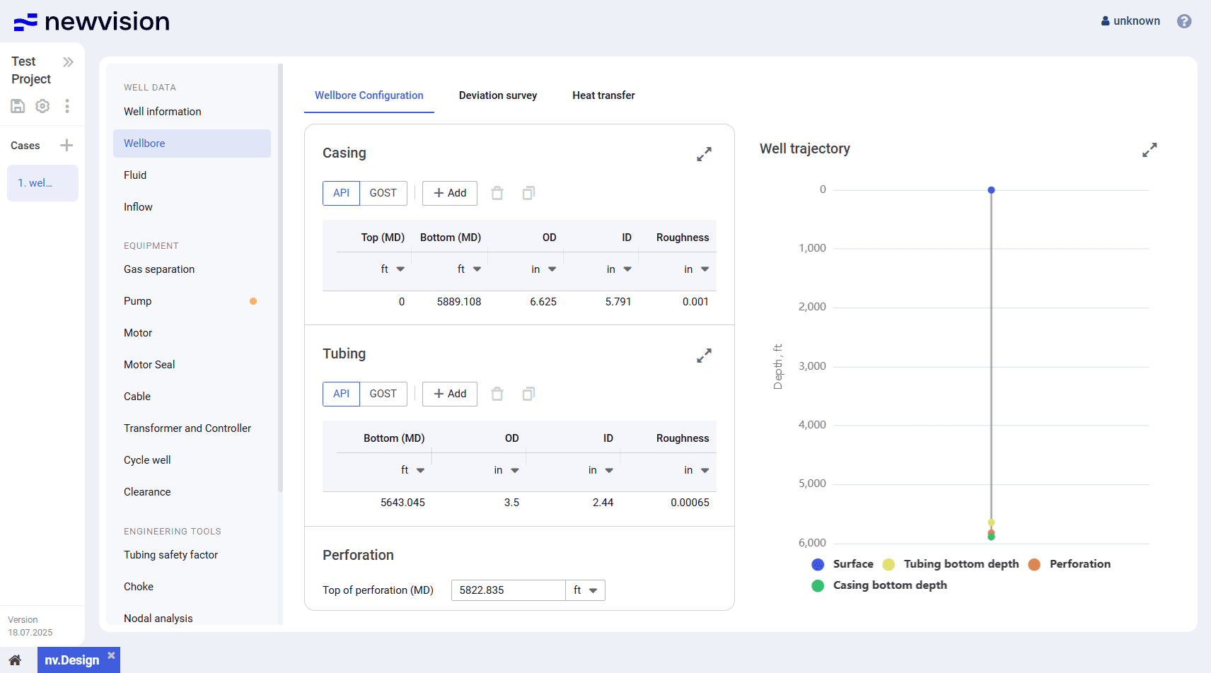 Select image to enlarge
- In the Casing parameter group, select the standard for outer and inner diameters of the casing: API or GOST .
Add new entries to the table. You can do it in the following ways:
To add a new entry, perform the following actions:
a. Above the table, click Add (
) .
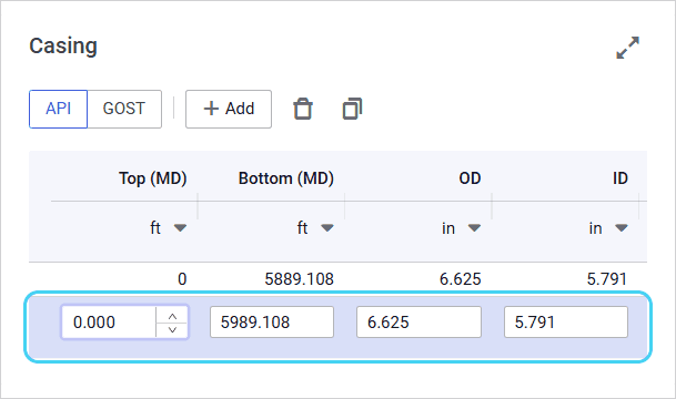
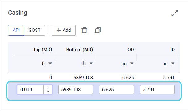
A new row appears in the table.b. In the new row, double-click values in the Top (MD) and Bottom (MD) columns and enter the desired values.
 Select image to enlarge
c. Double-click values in the OD and ID columns and select the desired outer and inner diameters from the lists.
To create a copy of an existing entry, select the entry that you want to copy in the table, and then, above the table, click Duplicate (
) .
The copied entry appears in the table.To paste a row with data from another table, copy it to the clipboard, select any entry in the table, and then press Ctrl+V.
The copied entry appears in the table.Scroll horizontally to view a wide table.Note
The inserted data must contain numerical values only. If the data includes a row with NaN (not a number) values, delete them after insertion.Entries in the table are automatically sorted by the Bottom (MD) value.
- Repeat Steps 3–4 for the Tubing parameter group.
In the right part of the Well Configuration tab, the well profile is displayed. (Optional)
To edit an entry, double-click the desired value and make necessary changes.
To delete an entry, select it in the table, and then, above the table, click Delete (
) .- To save changes, in the left part of the module, click Save (
 ) under the name of the current project.
5.1.2.2 Deviation survey#
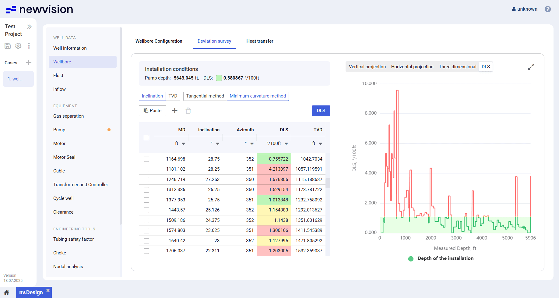
On the Deviation survey tab, you can build vertical, horizontal, dogleg severity (DLS), and 3D projections of the well.
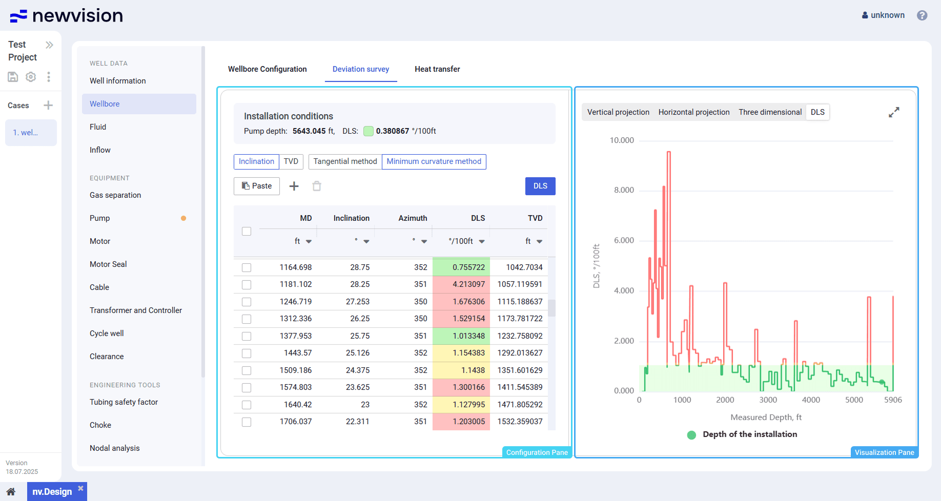
The tab consists of two panes:
- Configuration pane in the left part of the tab.
- Visualization pane in the right part of the tab.
 Select image to enlarge
Configuration Pane
The pane contains a table with the well directional survey data required for calculation. For details on how to enter the data and run a calculation, see Running Deviation Survey Calculation.
At the top of the pane, the installation conditions are displayed:
- Pump depth value equals the tubing bottom measured depth taken from the Wellbore configuration tab.
- DLS value corresponds to the dog leg severity at the pump setting depth. If there is no data for this very depth, the next available value is taken.
The color of the square to the left of the DLS value indicates if it is feasible to install the pump at this depth: a green square means that the maximum DLS value is withing the allowable range, a red one means that the maximum allowable value is exceeded. This value can be configured in the ESP depth setting determination window. For details, see Configuring DLS.
Below the Installation conditions area, the following controls are available:
Inclination / TVD
Provides the ability to select the parameter based on which the calculation will be performed.
In the table, values of the selected parameter are entered manually. Values of the other parameter are calculated automatically.
Tangential method / Minimum curvature method
Provides the ability to select the calculation method:
- The Tangential method assumes constant inclination and azimuth between survey points. Is simpler but less accurate.
- The Minimum curvature method models the well as a smooth arc and provides higher accuracy, especially over longer intervals.
By default, the Minimum curvature method is used as it offers the most reliable results for most wellbore profiles.
Paste (  )
)
Pastes data from the clipboard to a new row in the table.
Alternatively, to paste data, you can use the Ctrl+V shortcut.
| Note The inserted data must contain numerical values only. If the data includes a row with NaN (not a number) values, delete them after insertion. |
Add ( )
Adds a new row to the table for entering the deviation survey data. For details, see Running Deviation Survey Calculation.
Delete (  )
)
Deletes the selected rows from the table.
To select a row, select the corresponding check box in the leftmost column of the table.
DLS
Opens the ESP depth setting determination window where you can calculate the maximum allowable DLS values based on the ESP length and outer diameter. For details, see Configuring DLS.
In the table, values in the first three columns are editable. Values in the other two are calculated automatically.
In the DLS column, the following color indication is used based on the maximum allowable DLS:
- Green fill: The value is well below the critical value and no actions are required.
- Yellow fill: The value is 0,89-0,9 of the critical value and requires attention.
- Red fill: The value is greater than the critical value and must be fixed.
Visualization Pane
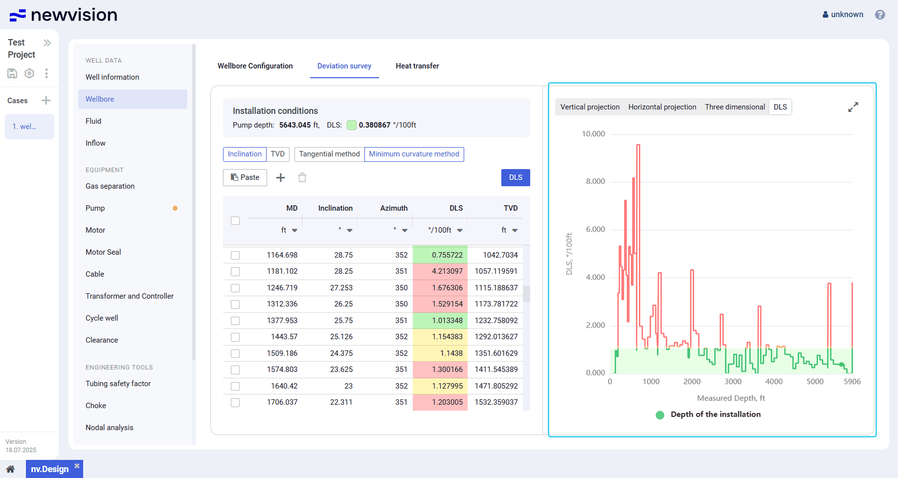
The pane provides the following types of the well projections distributed on the corresponding tabs:
- Vertical projection
- Horizontal projection
- DLS
- 3D projection
 | Important Projections are displayed only if the deviation survey data table in the left part of the section does not contain errors. |
 Select image to enlarge
On the DLS tab, sections suitable for equipment installation are highlighted with a green fill.
On other projections, depths are displayed as markers of different color.
To show or hide a marker, click its name under the profile.
You can also expand the pane to full screen or collapse it back to the original size using the Expand ( ) / Collapse ( ) buttons located in the upper-right corner of the pane.
5.1.2.2.1 Configuring DLS
To configure the well tubing and casing parameters, perform the following actions:
- Open the nv.design module.
For details on navigation in the system, see System Interface. In the left part of the working area, in the list of the module sections, click Wellbore , and then go to the Deviation survey tab.
 Select image to enlarge
At the top of the pane in the left part of the section, click DLS .
The ESP depth setting determination window opens in the right part of the section.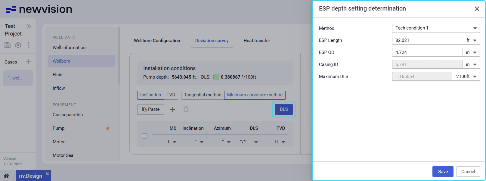 Select image to enlarge
In the window that appears, perform the following actions:
a. From the Method list select the calculation method: Tech Condition 1 (less strict) or Tech Condition 2 (stricter).
b. ( Optional) Edit values in the ESP Length and ESP OD fields.
Values in the Casing ID and Maximum DLS fields are calculated automatically.c. At the bottom of the window, click Save .
- To save changes, in the left part of the module, click Save ( ) under the name of the current project.
5.1.2.2.2 Running Deviation Survey Calculation
To configure deviation survey parameters and run a calculation, perform the following actions:
- Open the nv.design module.
For details on navigation in the system, see System Interface. In the left part of the working area, in the list of the module sections, click Wellbore , and then go to the Deviation survey tab.
Select image to enlargeAt the top of the pane in the left part of the section, select the parameter based on which the calculation will be performed: Inclination or TVD .
Scroll horizontally to view a wide table.Note
Values of the selected parameter must be entered in the table manually. Values of the other parameter will be calculated automatically.To the right of the parameters selected at the previous step, select the calculation method:
The Tangential method assumes constant inclination and azimuth between survey points. Is simpler but less accurate.
The Minimum curvature method models the well as a smooth arc and provides higher accuracy, especially over longer intervals.
Scroll horizontally to view a wide table.Note
By default, the Minimum curvature method is used as it offers the most reliable results for most wellbore profiles.- Above the table, click DLS and configure the maximum allowable dog leg severity. For details, see Configuring DLS.
Add new entries to the table. You can do it in the following ways:
To add a new entry, perform the following actions:
a. Above the table, click Add (
) .
A new row appears in the table.b. In the new row, double-click values in the first three columns and enter the desired values.
Values in the other two columns are calculated automatically.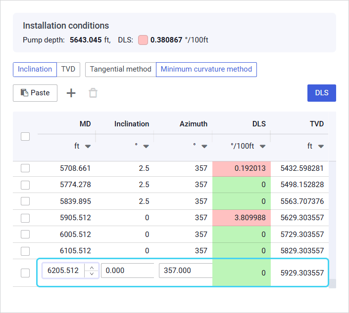 Select image to enlarge
To paste a row with data from another table, copy it to the clipboard, and then, above the table, click Paste (
) , or press Ctrl+V.
The copied entry appears in the table.Scroll horizontally to view a wide table.Note
The inserted data must contain numerical values only. If the data includes a row with NaN (not a number) values, delete them after insertion.- (Optional) To delete an entry from the table, select it, and then, above the table, click Delete ( ) .
Ensure that in the Installation conditions area above the table, the color of the square to the left of the DLS value is green. If it is red, make changes to the parameter values.
When the configuration is completed and there are no errors, in the right part of the tab, the well projections are displayed.
Select image to enlargeOn the DLS tab, sections suitable for equipment installation are highlighted with a green fill.
- To save changes, in the left part of the module, click Save ( ) under the name of the current project.
5.1.2.3 Heat transfer#
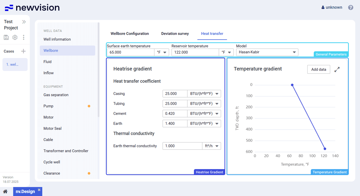
On the Heat Transfer tab, you can model the temperature distribution along the wellbore.
The tab consists of the following parts:
- General parameters at the top of the tab.
- Heatrise gradient pane in the left part of the tab.
- Temperature gradient pane in the right part of the tab.
 Select image to enlarge
General Parameters
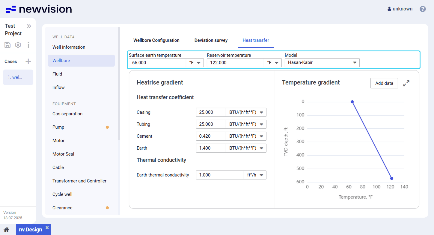
General parameters are required for the temperature gradient modeling.
 Select image to enlarge
There, you need to specify the Surface earth temperature and Reservoir temperature values and select the calculation model from the Model list.
Two calculation models are available:
- Hassan-Kabir: Provides more accurate estimates as it takes into account heat transfer coefficients of the well casing, tubing, cement, and formation, as well as thermal conductivity of the surrounding formation.
This method is based on a semi-analytical model developed by Hasan and Kabir, which solves the energy balance equations to estimate fluid and formation temperatures during steady-state or transient flow in the wellbore. - Rough Approximation: Provides less accurate but faster estimates. It requires fewer input parameters and uses only a general (lumped) heat transfer coefficient. This model is suitable for quick estimations or cases where detailed thermal data is unavailable. It generates a simplified temperature profile along the wellbore.
| Important If precise physical properties are not available, it is recommended to use the default Hassan-Kabir model. |
Heatrise Gradient
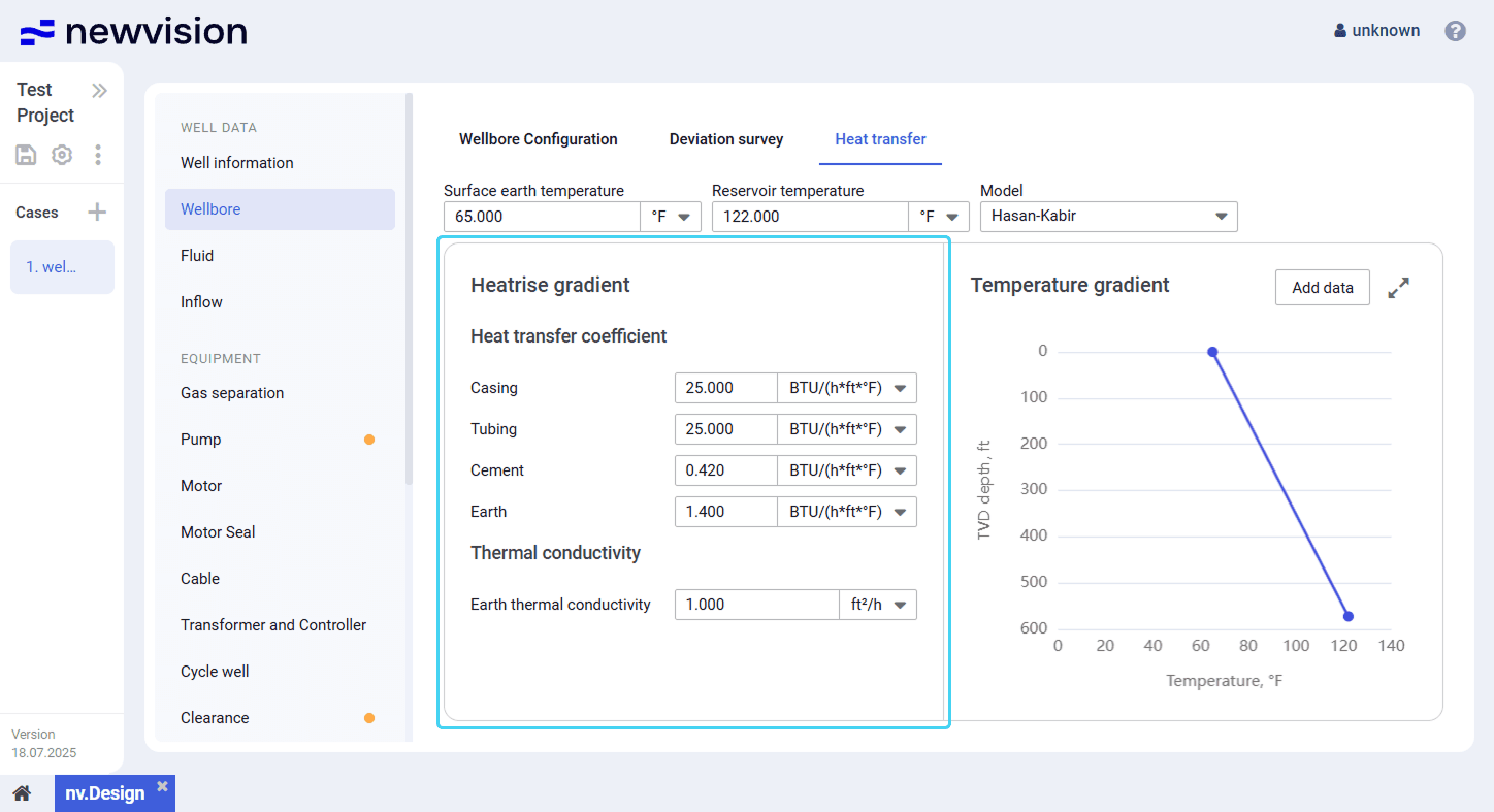
The pane contains well parameters that affect temperature distribution along the wellbore.
 Select image to enlarge
Depending on the selected model (see description above), different sets of parameters are available.
If the Hassan-Kabir model is selected, the pane contains two parameter groups:
- Heat transfer coefficient
- Thermal conductivity
If the Rough Approximation model is selected, only the Overall heat transfer coefficient value can be specified.
Temperature Gradient
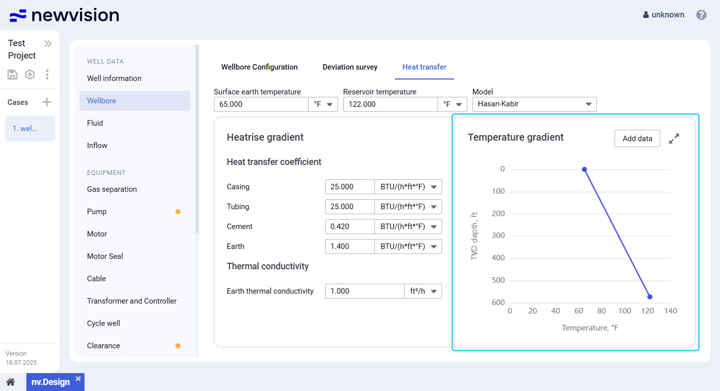
The pane contains a chart representing the well temperature profile constructed based on the input data and selected calculation model.
 Select image to enlarge
To improve the profile accuracy, you can add more information about the wellbore temperature at different depths. For details, see Adding Well Test Data.
You can also expand the pane to full screen or collapse it back to the original size using the Expand ( ) / Collapse ( ) buttons located in the upper-right corner of the pane.
5.1.2.3.1 Configuring Heat Transfer Parameters
To configure the well heat transfer parameters, perform the following actions:
- Open the nv.design module.
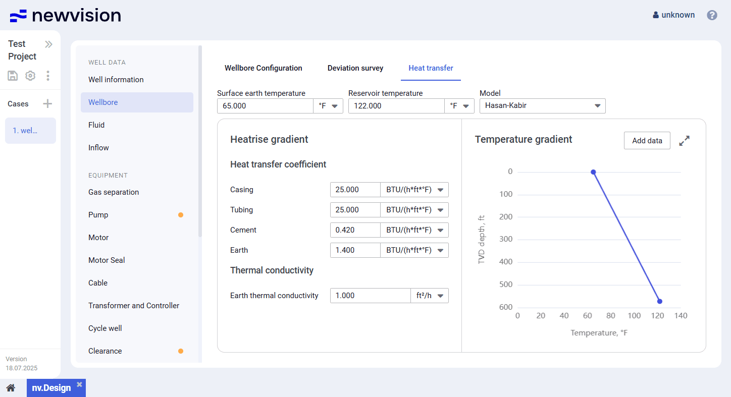
For details on navigation in the system, see System Interface. In the left part of the working area, in the list of the module sections, click Wellbore, and then go to the Heat transfer tab.
 Select image to enlarge
- At the top of the tab, in the Surface earth temperature and Reservoir temperature fields, enter the desired values.
- From the Model list, select the calculation model. For details, see Heat Transfer.
(Optional) In the Heatrise gradient pane, edit values of the desired parameters.
Scroll horizontally to view a wide table.Note
The list of parameters available in this pane may differ depending on the model selected in Step 4.- (Optional) To enhance the accuracy of the well temperature profile, in the upper-right corner of the section, click Add data and enter available temperature data at different well depths. For details, see Adding Well Test Data.
- After the configuration is completed, in the Temperature gradient pane, view the resulting temperature profile.
- To save changes, in the left part of the module, click Save () under the name of the current project.
5.1.2.3.2 Adding Well Test Data
To add temperature data obtained during the well tests, perform the following actions:
- Open the nv.design module.
For details on navigation in the system, see System Interface. In the left part of the working area, in the list of the module sections, click Wellbore, and then go to the Heat transfer tab.
Select image to enlargeAt the top of the pane, in the right part of the section, click Add data.
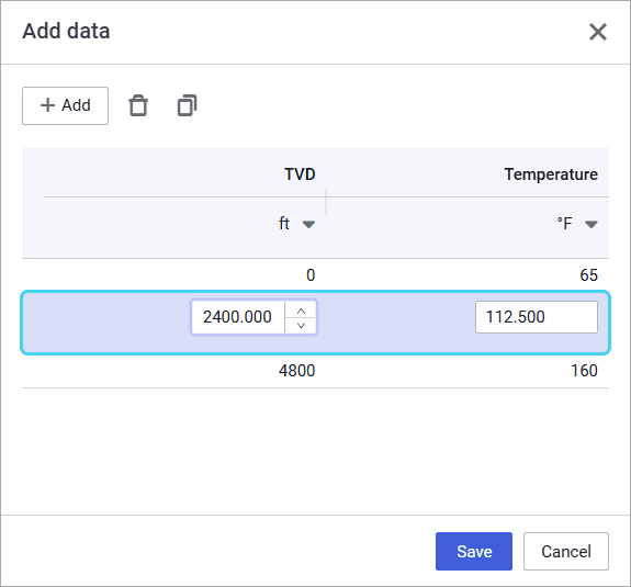
The Add data window opens in the right part of the section.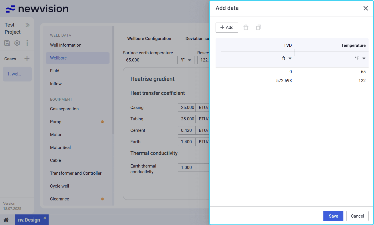 Select image to enlargeScroll horizontally to view a wide table.
Note
Two rows are added by default.
The first row is with a zero TVD and the temperature specified in the Surface earth temperature field at the top of the Heat transfer section.
The second row is with the TVD equal to the Top of perforation depth (MD) parameter from the Wellbore Configuration tab and the temperature specified in the Reservoir temperature field at the top of the Heat transfer section.Add new entries to the table. You can do it in the following ways:
To add a new entry, above the table, click Add (
), and then, in the new row, double-click values in the TVD and Temperature columns and enter the desired values.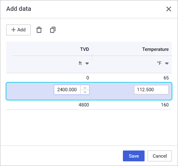 Select image to enlarge
To create a copy of an existing entry, select the entry that you want to copy in the table, and then, above the table, click Duplicate (
).
The copied entry appears in the table.- (Optional)
To edit an entry, double-click the desired value and make necessary changes.
To delete an entry, select it in the table, and then, above the table, click Delete (). - To save changes, in the left part of the module, click Save () under the name of the current project.